Friends RAG

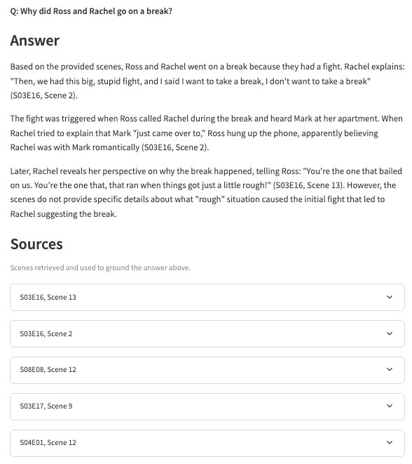
I built a RAG system that answers questions about the TV show Friends: It takes user’s question, scans through all 3,107 scenes of the show, selects 5 the most relevant ones, and serves them to LLM to answer the question based only on the information contained in the selected scenes. The creation of such a system itself is a clean process with good step-by-step guides. What was different, and where an interactive AI-assisted process pulls ahead of following a tutorial, is that my own results contradicted the standard playbook. Chasing down the why is what made this worth writing. The textbook answer for how to combine retrieval methods was not working well for this corpus. Catching that, locating the root cause, and addressing the issue is what this piece is about.

Summary

This project is a question-answering system over every episode of Friends, all 3,107 scenes of it. You ask a question, the system pulls the five scenes most likely to hold the answer, and an LLM answers from those five alone. Standing up that pipeline is well-trodden ground with good guides. The reason it was worth writing is that the standard advice failed on this corpus: the textbook move of fusing keyword search with vector search scored below plain keyword search, because fused as equals the weaker ranker dragged the stronger one down.

Most of the piece is working out why, and then fixing it. The cause was chunk size. Vector search was being handed whole scenes, too coarse for the kind of question people actually ask, and switching to a few-line window pulled it up to keyword search’s level. A larger embedding model and a tuned index search depth each added a few points on top. With both retrievers finally contributing, equal-weight fusion reached a recall@5 around 0.53, and a coverage experiment fixed the hard ceiling any reranker could reach at about 0.68.

The last real gain came from a reranker, a model that re-reads each candidate scene against the question and re-sorts them. Only one of the three I tested earned its place: Cohere’s reranker lifted recall@5 to about 0.62 and closed most of the gap to the ceiling, while the two open models barely moved it. What shipped is a live demo with two retrieval modes, a fast hybrid by default and the reranker behind a toggle, running on a free Hugging Face Space. Underneath the retrieval work, the project was also a test of how far a product manager can get building hands-on with an AI coding partner, and of where that partnership starts to strain over a long, stateful build.

Why build this, and why Friends

As a Product Manager, the most useful reason to build things myself is what it does for my conversations with engineers: they become more meaningful and impactful. The broader reason is that the barrier is now low enough that hands-on building is becoming table stakes for non-engineers in general.

As a side quest, I wanted to test how far “assisted engineering” (Andrej Karpathy’s term for coding with an AI partner doing the heavy lifting) goes with today’s capabilities. Whatever the ceiling is nowadays, I didn’t hit it this project. More on that in What I learned.

Friends turned out to be a good corpus for three reasons:

• It’s large and varied. Some questions are isolated to one moment (“Why did Ross shout PIVOT?”), others are distributed across the whole series (“Name all of Chandler’s girlfriends”). That range stresses a retrieval system in different ways.
• It’s demoable. People know the show, so the demo sparks engagement instead of polite nods.
• I’ve watched the show so many times that I can judge almost any answer instantly without looking anything up.

The dataset comes from the Character Mining project by Emory NLP, and it’s excellent: clean, verified text with per-utterance speaker labels and even stage directions.
The part that mattered most for my project is that it ships with a built-in span_qa question-and-answer set, known questions paired with the exact utterances that answer them. That’s what made evaluation possible without me hand-labeling hundreds of examples.
The full corpus is 236 episodes, 3,107 scenes, 67,373 utterances, roughly 1.1M tokens.

Tools

Claude Code did the heavy lifting: co-author, engineering partner, and a surprisingly good research consultant.
Cursor handled refactors, code explanations, and file manipulation.
Terminal was for environment management, small script edits, running things, and git.

Basics: RAG, chunking, vector vs. keyword retrieval, and the metrics

RAG (Retrieval-Augmented Generation). Instead of asking an LLM to answer from its training, you first retrieve the most relevant chunks of your own text and put them in the prompt: “Here are five relevant passages. Answer using only these.” The model contributes language and reasoning; the retrieved documents contribute facts.

Chunking. Before any retrieval, the source text is split into smaller pieces - chunks. A chunk is the unit that gets embedded, indexed, and ultimately retrieved. Chunk size is a design choice. Too large, and one chunk covers many topics, diluting the signal for any single one. Too small, and it loses the surrounding context that gives a line its meaning. This choice becomes central later.

Vector retrieval. Each chunk is passed through an embedding model that turns it into a vector (a long list of numbers) capturing its meaning. Semantically similar text lands close together in that multidimensional space. To retrieve, you embed the question the same way and find the nearest chunks by distance (L2 or cosine). Strength: it matches meaning, so “how do I cancel my plan” finds “steps to terminate a subscription.” Weakness: it can blur specific rare terms.

BM25 (keyword retrieval). The classic keyword-ranking algorithm behind decades of search boxes. It rewards passages that contain the question’s words, weights rare words far more heavily than common ones, and corrects for length so a long passage doesn’t win just by having more words in it. It excels at exact rare terms and fails on pure paraphrase: if the question and the text share no words, BM25 can’t connect them.

	Vector	BM25
Matches	meaning / paraphrase	exact terms
Great at	”where do they hang out"	"Nina Bookbinder”
Blind to	precise rare tokens	synonyms / rewording

recall@k is the headline metric here. Of the questions where a correct source scene exists, it’s the fraction where at least one correct scene shows up in the top k retrieved results. I report recall@5. Why this metric: it maps directly to “did the system hand the LLM a scene from the right episode?” If the right scene never makes it into the context, the generated answer can’t be correct, so recall@5 gates everything downstream.

MRR (Mean Reciprocal Rank) is a supporting signal. It rewards ranking the correct scene higher (rank 1 is worth more than rank 5), not just including it somewhere. I used it in evaluation as a supplementary metric.

References: RAG (Lewis et al., 2020) · embeddings / vector search · BM25 (Wikipedia) and the canonical write-up, Robertson & Zaragoza, “The Probabilistic Relevance Framework: BM25 and Beyond” · recall and MRR (evaluation measures)

Tech stack

The stack is quite standard:

• Embeddings: OpenAI model: text-embedding-3-small, produces 1536 dimensions vectors.
• Vector store: Chroma, queried by L2 distance.
• Keyword search: rank_bm25, a small Python library implementing the BM25 family (b=0.75 is the standard setting for how much it discounts longer passages).
• Fusion: Reciprocal Rank Fusion (RRF), a standard way to merge two ranked lists using only each item’s rank position, not its raw score; k=60 is the conventional smoothing constant that keeps any single top result from dominating.
• Generation: Claude (model: claude-haiku-4-5), instructed to answer only from retrieved scenes, cite them, and refuse when they’re insufficient.
• Retrieval depth: top-5.

The rest is plumbing: JSONL files and common Python libraries like chromadb for the vector store and sentence-transformers for the reranking models.

GitHub repo: github.com/peselev/friends-rag

The pipeline

Specifically here the pipeline loads the raw Emory JSON (130MB), strips each utterance down to the essentials (ID, speaker, transcript), and emits a roughly 5MB processed file. From there it chunks and embeds the text into Chroma, builds the BM25 index. At query it retrieves from both, fuses, and generates the answer. Evaluation isn’t part of this runtime path; it was a separate activity I ran while tuning the pipeline, and it’s the subject of the next section.

See it in action

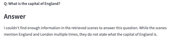
A few moments that show the behavior I cared about most: answering from the scenes it found, and knowing when to stop.

Answering a question, with the scenes it used expanded underneath.

Refusing a question the show can’t answer, instead of inventing one.

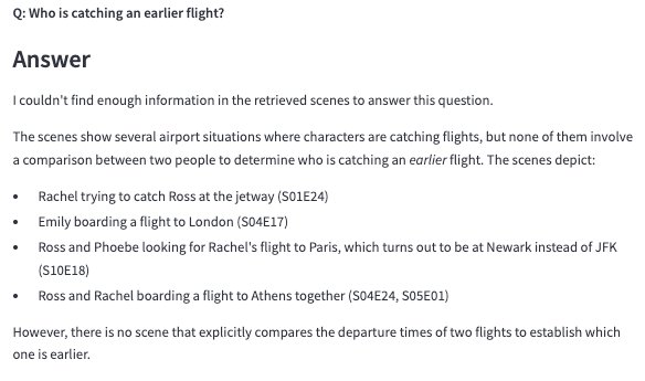
Admitting when the retrieved scenes don’t contain enough to answer.

Evaluation

Seeing the feature working is an emotional milestone, but of course, it’s not the completion of the project: in traditional programming it can be misleading due to bugs, unaddressed edge cases, wrong configuration etc. But in probabilistic software the question is not only “does it work” (did it generate the answer), but “is it helpful” (is the answer correct, is it correct for the right reasons?)

To evaluate the performance of my RAG I was using the Q&A dataset included in the Character Mining dataset. First, I built several modes for retrieval:

1. Scene-long vector (1 chunk is a scene in the episode)
2. BM25 (search by keywords)
3. Hybrid (each retriever ranks the chunks on its own, then Reciprocal Rank Fusion blends the two ranked lists into a single ordering)

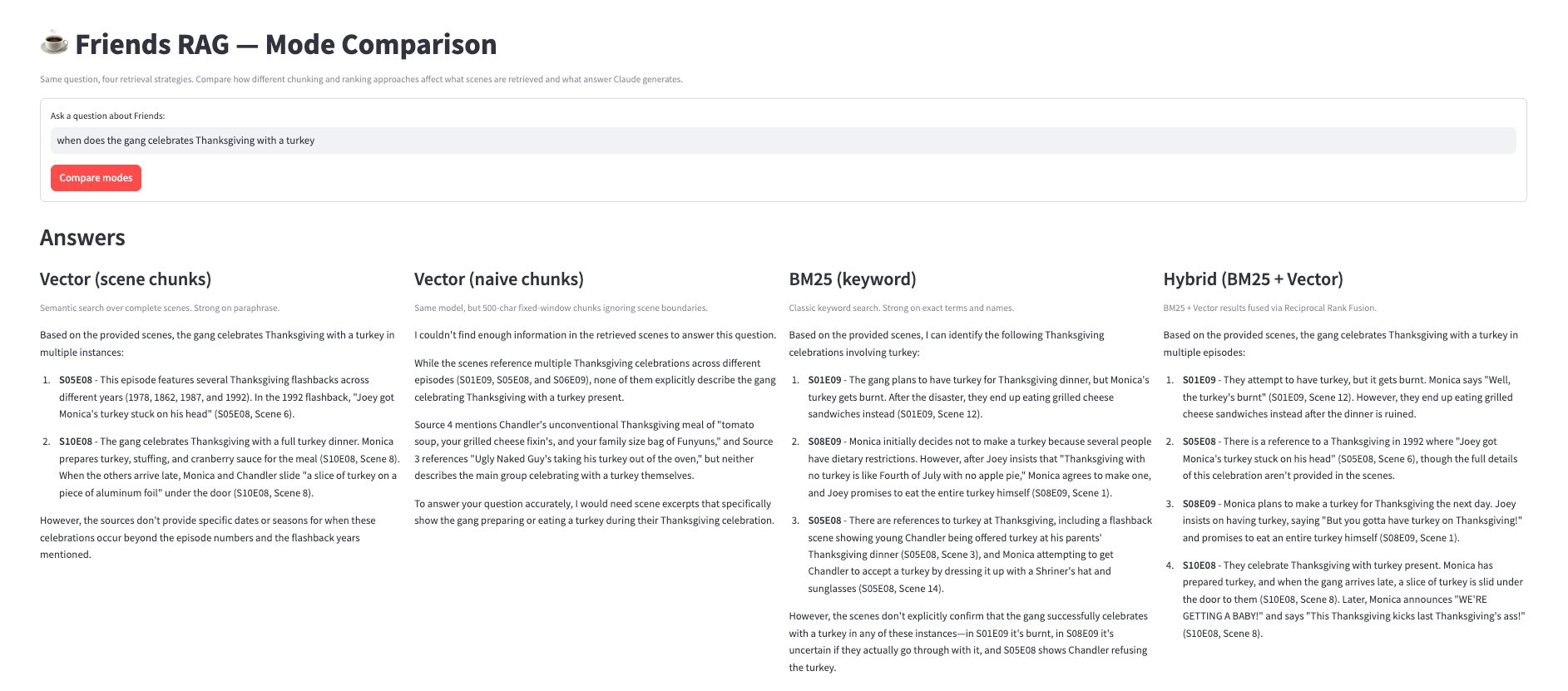
(↗Click to enlarge) A local tool I built to see how each retrieval strategy answers the same question, side by side.

The method is straightforward, because the dataset does the hard part. Every span_qa question comes paired with the exact utterances that answer it, so for each question I already know the correct scene. I ran each question through every mode, took the top five results, and recorded whether a correct scene appeared (recall@5) and how high it landed (MRR). I ran this on the original questions and on Emory’s paraphrased versions of them.

I evaluated at this point, before polishing generation or the interface, on purpose. Retrieval is the gate. If the right scene never enters the context, no amount of prompt tuning or interface work can make the answer correct. Measuring retrieval first tells me whether anything built on top of it can succeed at all.

The common tutorial framing goes roughly like this: dense vector retrieval, enabled by transformer models, is the modern default and generally beats classical keyword search when compute isn’t the constraint; and adding keyword search on top, as a hybrid, usually improves precision beyond either method alone.
This framing is common in practitioner guides, but it’s contested in the literature: dense retrieval’s edge is workload-dependent, and BM25 remains a strong baseline on many benchmarks (e.g. BEIR), sometimes beating dense retrieval outright on domain corpora with precise terminology (T2-RAGBench, 2026). The “hybrid beats either alone” half is well supported but, as this project shows, not automatic.

Retrieval mode	Direct (recall@5)	Reworded (recall@5)
BM25 (keyword)	0.453	0.470
Vector (scene-level)	0.300	0.357
Hybrid (scene-level vector + BM25)	0.367	0.405

What “Direct” and “Reworded” mean

Throughout this write-up I test against the same questions worded with progressively fewer of the script’s literal words. Direct questions are taken as written from the dataset. Reworded questions are the dataset’s own paraphrases, which change the phrasing but keep the key names intact. Here is one scene with a direct and a reworded question about it:

Carol: Anytime you’re ready.
Ross: Ok, ok, here we go. (he crouches down near her stomach) Ok, where am I talking to, here?
Carol: Just aim for the bump.
Ross: …this is too weird. I feel stupid.
Carol: So don’t do it, it’s fine. You don’t have to do it just because Susan does it.
Ross: (quickly talking) Hello, baby. Hello, hello.

• Direct: “When does Carol tell Ross to talk to the baby?”
• Reworded: “At what moment does Carol invite Ross to start speaking to the baby?”

Both keep “Carol,” “Ross,” and “baby,” the exact terms BM25 leans on.

However, the textbook recipe stumbled here, on both counts. Whole-scene vector search was the weak link at 0.300 on direct questions, well below BM25’s 0.453. And the hybrid, which is supposed to be the safe choice, came in at 0.367, under BM25 alone: fusing the two as equals let the weaker ranking pull the stronger one down instead of combining their strengths. The reworded questions came out the same way (0.357 and 0.405 against BM25’s 0.470), because Emory’s paraphrases keep the proper names BM25 keys on, so keyword search never lost its footing.

So I had a baseline and a problem. The modern method had lost to the classical one, and the hybrid had made things worse instead of better. Either dense retrieval was the wrong tool for a corpus of short, name-heavy dialogue, or I was feeding it the wrong input. Separating those two was the next phase.

Improving

My best recall@5 so far is 0.453 for Direct questions, and 0.470 for Reworded questions. One way to interpret it is that for more than a half of questions the retriever did not serv the right scene in its top 5 scene list. This doesn’t translate 1:1 into bot not having right information more than half of the time (the answer might be still contained in a different scene that was not marked as the correct one). However, there is still a correlation, and genersally speaking, the higher recall@5, the more useful the bot will be.

Use different chunks

What if the chunk sizes I tried were too far from the sweet spot? Every article about RAG goes out of its way to explain how critical chunk size is.

What I tested, and what came back

A typical FriendsQA question targets a tiny exchange: “What does Julio say to Jeannine?” is about five seconds of screen time. But I had embedded whole scenes, sometimes 50 utterances long. Inside a single scene vector, the “Julio” moment is one idea competing with everything else in the scene, so the scene’s vector barely resembles the question even when the answer is sitting inside it. BM25 doesn’t have this problem, because it keys on the rare token “Julio” wherever it appears.

So, I tested finer chunks against the scene baseline.

Retrieval mode	Direct (recall@5)	Reworded (recall@5)	Δ vs scene (Reworded)
Vector (scene-level)	0.300	0.357	baseline
Vector (single utterance)	0.268	0.265	−0.092
Vector (5-utterance window)	0.440	0.472	+0.115

Result: granularity was the dominant lever. The 5-utterance window beat scene-level by a wide margin, +0.140 on direct questions and +0.115 on reworded, which pulled the best vector mode up to BM25’s level (0.440 and 0.472 against BM25’s 0.453 and 0.470). Going finer backfired: single utterances scored below whole scenes (−0.092 on reworded), because a line stripped of its surrounding exchange loses the context that tells the embedding what it is about. A window of a few lines was the size that matched a typical question, enough to isolate the answer without losing it inside a whole scene. This answered the question the first results had raised: dense retrieval was not the wrong method for this corpus, I had been feeding it the wrong chunk size.

Use a larger embedding model

The ceiling can be theoretically lifted with a more powerful embedding - regardless of the chunk size, or fusion technique, a higher dimensional space should provide the increase in recall@k metric, since it captures the relevance between the question and scenes better. I had been using OpenAI’s text-embedding-3-small - it’s cheap and fast, mostly because it’s the cheap default. An obvious experiment: re-embed the entire corpus with text-embedding-3-large (twice larger) and measure what changes.

What I tested, and what came back

I built a parallel set of Chroma collections embedded with text-embedding-3-large (3072 dimensions, versus 1536 for small) and re-ran the exact same union-coverage experiment against them — same chunks, same questions, same harness. The only thing that changed was the embedding model. BM25 was left in as a control: it uses no embeddings, so if the harness is clean its numbers must not move at all.

Reference: OpenAI embedding models

The control behaved exactly as it should — BM25 was identical to the third decimal across every question set, which told me every other number below is a real embedding effect and not measurement noise. And every vector mode did improve:

Mode	Set	Small	Large	Δ
Scene	Direct	0.285	0.370	+0.085
	Reworded	0.350	0.372	+0.022
Window	Direct	0.430	0.530	+0.100
	Reworded	0.470	0.512	+0.042
Single utterance	Direct	0.268	0.310	+0.042
	Reworded	0.253	0.350	+0.097
BM25 (control)	Direct	0.453	0.453	0.000
	Reworded	0.470	0.470	0.000

The gains were real but modest, and uneven across modes and question types. The window mode, the one I actually rely on, picked up the most on direct questions, +0.100 to 0.530, but only +0.042 on reworded. Single utterances gained most on reworded (+0.097) and little on direct. Scene moved least, and its reworded gain (+0.022) sits inside the run-to-run wobble of the default-ef index. A bigger embedding bought a handful of recall points, spread unevenly across modes. I decided the larger model was not worth adopting. It doubles the vector dimensions (3072 against 1536), so it doubles storage and memory, costs several times more per token to embed, and adds latency to every query as a permanent cost. Against that, a handful of unevenly distributed recall points is a weak return, especially next to the cheaper levers in this project: the chunk-size change alone was worth more than this, and search-depth tuning and fusion were still ahead of me, both free. I measured this before tuning Chroma’s search depth and did not revisit it afterward, since the case against the larger model never rested on a few points of recall. I stayed with text-embedding-3-small, treating the larger model as a lever I could pull later if I ever needed the last points.

Fine-tune Chroma search depth

This one started as a discrepancy I couldn’t explain. Two of my own evaluation scripts disagreed about the same vector modes: on identical questions, with an identical metric, one reported a few points higher recall than the other. The only thing that differed was how many candidates each pulled from Chroma before scoring. BM25 matched exactly across both, and so did the small scene-level collection. The gap showed up only on the large window and utterance collections, the ones holding tens of thousands of vectors.

That pattern has one explanation. Chroma stores vectors in an HNSW index, which finds nearest neighbors approximately rather than comparing a query against every vector in the collection. How hard it looks is governed by a parameter called search_ef, and the answer gets more accurate the more candidates you ask it for. The script that fetched deeper was landing closer to the true nearest neighbors; the one that fetched shallow was settling for a rougher approximation. On a 3,000-vector collection that approximation is nearly exact and the difference is invisible. On the 61,000-vector window collection it was quietly costing real recall.

How I measured it, and what came back

I rebuilt the window collection at a range of search_ef values, held the fetch depth fixed, and recorded both recall@5 and per-query latency at each. Because search_ef is locked in when a collection is created (changing it afterward has no effect in this version of Chroma), I pulled the existing vectors out of each collection and re-added them under the new setting, rather than paying to re-embed the whole corpus.

search_ef is Chroma’s query-time HNSW search-depth setting; higher values search more of the index.

The window mode, recall@5 on direct questions, against median query latency:

search_ef	recall@5	median latency
default	0.435	2.8 ms
100	0.458	3.0 ms
200	0.472	4.3 ms
400	0.487	6.3 ms
800	0.492	9.2 ms

Recall climbs steeply, then flattens. By search_ef=400 the window mode has recovered almost all the way to its exact-search ceiling of about 0.49, and the step up to 800 buys almost nothing. The price is a few milliseconds per query, which is negligible against the rest of the pipeline: generation runs in the hundreds of milliseconds, and the reranker, when it is on, adds seconds. I set search_ef=400 on every collection and made it the default in the indexer. (Reworded questions tracked the same curve, reaching 0.497 at search_ef=400.)

One effect doesn’t show up in the table. The live demo fetches fewer candidates per query than this experiment did, so its searches were running even rougher than the default row suggests. Pinning search_ef=400 helps the deployed app more than it helps the benchmark. And it wasn’t really an optional tweak: the under-searching had been suppressing every vector and hybrid number until I caught it, which is why the vector results throughout this writeup are all measured with this setting in place.

Estimating the ceiling for the retrieval

All the previous steps were ON/OFF decisions:
The larger embedding gave only a modest lift (a few points of recall@5, uneven across modes), not enough to justify its cost, so I stayed with the cheaper model.
Similar approach was relevant while tuning Chroma index’s search depth search_ef:

• If deeper search had introduced significant latency with negligible improvement, I could have reverted to the default.
• If the latency and the lift had both been significant, I could have reserved a deepaer search mode for a special “more accurate” setting.
• Since it turned out to be a clear win with no significant downsides, I settled on an optimal value (400).

However, the next steps were different. I planned to apply two techniques to improve the quality:

1. Optimize the fusion
2. Introduce the reranker

The details about each of the two are below in their respective sections. Neither of these ideas had an obvious bar to clear: how “good” was “good enough”? With a given lift, how far away am I from the maximum? Thus, before proceeding further, I needed to estimate a theoretical ceiling for the accuracy:

What I measured, and why it is the real ceiling

A retriever can only rank scenes it actually pulled back. Fusion reorders them and a reranker reorders them, but neither can surface a scene that no retriever returned. So the true ceiling on recall is the union: for each question, pool everything all four retrievers found and ask whether the correct scene is in that pool at all. If it is not there, nothing downstream can recover it.

I ran every question through all four retrievers (BM25, scene, window, single utterance), took a deep slice of each, and pooled them into one candidate set. Then I measured coverage at growing depths: for what fraction of questions does the correct scene appear anywhere in the pooled top 5, 10, 20, or 50. The top-5 figure is the most a perfect fusion could reach; the deeper figures are what a reranker could reach if it were handed that many candidates and ordered them perfectly.

Pool	Set	@5	@10	@20	@50
BM25 alone	Direct	0.453	0.525	0.590	0.660
	Reworded	0.470	0.535	0.580	0.642
BM25 + window	Direct	0.600	0.655	0.725	0.800
	Reworded	0.593	0.657	0.715	0.765
BM25 + window + scene	Direct	0.623	0.682	0.748	0.830
	Reworded	0.625	0.690	0.738	0.775
Full pool (all four)	Direct	0.640	0.695	0.752	0.840
	Reworded	0.660	0.713	0.760	0.795

Pooling all four retrievers, the correct scene is reachable for 64% of direct questions in the top 5, climbing to 75% at top 20 and 84% at top 50 (reworded tracks close: 66%, 76%, 80%). Almost all of that comes from BM25 and the window vector together; adding the scene and utterance vectors lifts the ceiling by only three or four points, because they mostly re-find scenes the strong pair already covers. The gap between this ceiling and what a single fused ranking puts in the top 5 (around 0.55, measured next) is the headroom a reranker can chase, since reordering a deep pool can only ever surface scenes the pool already holds.

Adjust the fusion of different retrievers together

The naive hybrid fuses BM25 and the window vector with equal weight, the simplest possible choice, but not an obviously correct one. If one retriever is stronger, maybe its vote should count for more. And I still had two retrievers sitting unused, the scene and single-utterance vectors, which might widen the net. So I tested two questions: whether a smarter weighting beats equal weight, and whether fusing all four retrievers beats fusing the best two. Beyond naive I tried two weighting schemes, a fixed weight and a query-aware dynamic weight, on both the two-retriever pair and the full four.

How the query-aware weighting worked

All the fusion modes use Reciprocal Rank Fusion. Each retriever ranks its scenes, and a scene’s combined score is the sum across retrievers of 1 / (k + rank), so a scene ranked high by either retriever rises and one ranked high by both rises most. No score normalization is needed, which is part of why RRF is a common default. The modes differ only in how much each retriever’s vote is weighted. Naive gives every retriever equal weight. Fixed uses one static weight for all queries: I swept a few splits and kept the best, which leaned toward the window vector, the stronger of the pair. The dynamic mode adapts the weight to each query using inverse document frequency, the standard measure of how rare a term is across the corpus. A query full of distinctive proper nouns scores high and leans toward BM25, which keys on exact rare words, while a query of common words leans toward the vector side. The premise was that no single fixed weight can serve both kinds of query, but an adaptive one might.

References: inverse document frequency (IDF) · Reciprocal Rank Fusion (Cormack et al., SIGIR 2009)

Fusion mode	Set	@5	@20	@50
BM25 + window, naive	Direct	0.530	0.675	0.757
	Reworded	0.507	0.675	0.730
BM25 + window, fixed	Direct	0.550	0.655	0.720
	Reworded	0.520	0.640	0.685
BM25 + window, query-aware	Direct	0.545	0.655	0.725
	Reworded	0.525	0.640	0.688
All four, naive	Direct	0.510	0.652	0.743
	Reworded	0.482	0.660	0.740
All four, fixed	Direct	0.542	0.670	0.752
	Reworded	0.522	0.647	0.743
All four, query-aware	Direct	0.527	0.667	0.738
	Reworded	0.510	0.650	0.725

Weighting toward the stronger retriever did help at recall@5, but only by about two points: 0.550 for the fixed weight and 0.545 for the query-aware one, against 0.530 for naive on direct questions. The two weighted modes tied, which is itself a result. The query-aware version, for all its per-query machinery, did no better than a single static weight, so the adaptivity earned nothing on this corpus. (And the fixed weight was tuned on the same questions it was scored on, so even its small edge is an optimistic one.)

The more useful finding is deeper in the list, and it comes back to what fusion is for. Fusion buys two things: consensus, where both retrievers agree a scene is relevant, and coverage, the pooling of both lists so that more candidate scenes get a chance at all. Weighting trades one for the other. Tilting toward the strong retriever sharpens the top of the list, which lifts recall@5, but it pushes the weak retriever’s unique finds below the cutoff, which costs coverage. So the ranking inverts: the weighting that wins at recall@5 loses at recall@50, where naive equal weight is best (0.757 against 0.720). Equal weight maximizes coverage; weighting maximizes precision at the very top.

Fusing all four retrievers did not help the final ranking. At recall@5 the four-way pool was no better than BM25+window, and the naive four-way was worse, because the two weaker vector modes mostly re-find scenes the strong pair already has (the ceiling experiment showed they add only a few points even to the union). As equal voters, they mostly pushed noise into the top of the list.

So there was no single best fusion, only a best one for each use. Weighting toward the window vector gives the best recall@5, which is what the fast retrieval mode wants. But it costs coverage deeper in the list, so for the candidate set that feeds the reranker, where coverage matters more than order because the reranker re-sorts it anyway, equal weight is the better choice. Which weighting wins depends on how deep the next stage reads, and the next stage is the reranker.

Add a reranker step

A reranker is a second pass. The idea is the following: if different retrievers find the right scene for different questions, then recall@5 might get improved, if I find a way to benefit from that extended coverage. At the same time, if different retrievers find the same right scenes, recall@5 might get improved from consensus between retrievers. Moreover, having a fusion mechanism that elevates correct scenes would let me retrieve deeper (k=10, 20, or even 50) and still elevate the right scenes, using the diversity of the retrievers. The problem, of course, is that serving dozens of scenes to the LLM hoping it will see the relevant data there would (a) confuse the LLM, not help it and (b) increase the cost (beating the whole point of RAG).

The right approach is not to serve more to LLM, but to rank the scenes better: The first stage retrieves a short-list of candidates quickly; the reranker, a cross-encoder, then reads the question and each candidate together and scores how well they actually match.

More about the cross-encoder

The difference from first-stage retrieval is what the model looks at. The vector retrieval in stage one embeds the question and each passage separately, ahead of time, and compares the finished vectors. A cross-encoder embeds nothing in advance: it takes the question and one candidate passage together as a single input and outputs one relevance score for that pair. Because it can attend to both texts at once, it judges relevance far more precisely. The cost is that nothing can be precomputed, so it has to run fresh for every question-candidate pair at query time, which is why it only runs on a short list of candidates rather than the whole corpus.

References: cross-encoders and the retrieve-then-rerank pattern (Sentence Transformers docs)

The standard recipe is to retrieve a wide top-N, rerank, and keep the top five. I expected a clean lift in both recall and ranking.

I tried two open models, MS-MARCO MiniLM and BGE, and one paid - Cohere.

The full results, floor to ceiling

Retrieval mode	Set	recall@5	MRR (Direct)
Hybrid, no rerank (floor)	Direct	0.530	0.431
	Reworded	0.507
+ MS-MARCO MiniLM	Direct	0.537	0.455
	Reworded	0.545
+ BGE	Direct	0.552	0.473
	Reworded	0.568
+ Cohere	Direct	0.620	0.533
	Reworded	0.625
Ceiling (ideal reranker)	Direct	0.675	0.675
	Reworded	0.675

The lift came almost entirely from one model. At the production depth, twenty candidates fed to the reranker and the top five kept, Cohere’s rerank-v3.5 raised recall@5 from 0.530 to 0.620 on direct questions and from 0.507 to 0.625 on reworded ones, a gain of roughly nine to twelve points. It also led on ranking quality, with MRR on direct questions climbing from 0.43 to 0.53. The two open cross-encoders barely touched the direct number: MiniLM added under a point, BGE about two. Both did more for the reworded set, four to six points, but neither came close to Cohere on either.

The split traces back to what each model was trained on. MiniLM and BGE learned relevance from MS-MARCO, a corpus of web passages, which transfers poorly to short lines of sitcom dialogue. And these questions lean heavily on proper names, the signal BM25 already ranks well, so a weak cross-encoder has little room to improve on the fused order. Only the stronger model knew the domain well enough to reorder the candidates better than the fusion had.

Pulling more candidates did not help, which turned out to be the more useful result.

The full depth comparison, N=20 vs N=50

Mode	Set	N=20	N=50
Hybrid, no rerank (floor)	Direct	0.530	0.530
	Reworded	0.507	0.507
+ MS-MARCO MiniLM	Direct	0.537	0.542
	Reworded	0.545	0.537
+ BGE	Direct	0.552	0.560
	Reworded	0.568	0.547
+ Cohere	Direct	0.620	0.635
	Reworded	0.625	0.620
Ceiling (ideal reranker)	Direct	0.675	0.757
	Reworded	0.675	0.730

recall@5 with N=20 vs N=50 candidates fed to the reranker. The floor doesn’t depend on N; the ceiling is the share of questions whose gold scene is anywhere in the fused pool.

The table moves the wrong way for depth. The ceiling climbs about eight points on direct questions, but every reranker stays nearly flat and the reworded numbers slip. A deeper pool is also a noisier one, and a model that cannot cleanly sort the noise just finds more ways to put the wrong scene first. So the headroom grows instead of closing: after Cohere reranks twenty candidates, 0.055 of direct questions have a reachable gold scene stuck below the top five, and at fifty that remainder more than doubles to 0.122. Twenty is the operating point.

That contrast is the honest read on where the bottleneck sits now. The 0.675 ceiling in these tables is the naive hybrid’s recall@20 from the fusion section, since the reranker only reorders the twenty candidates it is handed and can never surface a scene that pool doesn’t hold. At twenty candidates Cohere reaches 0.620 of that 0.675, closing about three-fifths of the gap above the no-rerank baseline. The misses that remain split in two: some are scenes no retriever returned at all, which no reranker can recover, and some are scenes sitting in the candidate pool that the reranker still orders too low to reach the top five. The second kind is what a stronger reranker could keep chasing. Retrieval coverage is no longer the only thing holding the number down.

Settling for the retrieval mode for demo

The demo ships two modes, and the split follows the numbers. The default is the fast naive hybrid: BM25 fused with the window vector, top five, no reranker. It returns in a couple hundred milliseconds, costs nothing per query, leans on no outside service, and at recall@5 near 0.53 it already answers the questions most visitors will ask. For a public demo that should feel instant and never stall waiting on an API, that is the right default.

The second mode, behind a “higher accuracy” toggle, adds the Cohere reranker. Cohere was the only reranker that earned its place in the experiment, lifting recall@5 to about 0.62, so it is worth offering. It is also a paid API call, slower and metered, and it leans on a service I do not run. Those are reasonable costs when someone deliberately asks for the better answer, and poor ones to put on every default query, so Cohere lives behind the toggle. This is also why the toggle no longer uses the open BGE model it shipped with: the experiment showed BGE barely moved recall, and Cohere was the only model that did.

The toggle changes one thing besides the model: it retrieves a deeper pool. The fast mode keeps the fused top five and stops. The reranked mode keeps the fused top twenty and hands all of them to Cohere, which re-sorts them and returns the best five. The depth is the point, because a reranker can only reorder what it is handed. Given five candidates it could do nothing for recall@5, since the set is already fixed at five. Given twenty, it has room to lift a correct scene from rank six through twenty into the top five, which is where its gain comes from.

Because the reranked mode depends on an outside service, it degrades gracefully. It defaults to a free Cohere trial key, falls back to a production key if the trial key is rate-limited or out of its monthly allowance, and if Cohere is unreachable for any reason it skips the rerank and serves the fast hybrid result with a short note. The toggle can get slower or quietly become the fast mode; it does not break the demo.

None of that confidence would have meant much without a final, untouched test.

The holdout test

Before committing, I ran a holdout test. Early on I had set aside a sealed set of hand-curated questions about who Joey was in love with, a deliberately hard case because the evidence is spread across many episodes and the show never states it outright. I wrote down the expected answers in advance and committed them to the repo before running the final test, so the timestamp proves I didn’t move the goalposts. Then I ran the set once. The three questions, narrowing from broad to specific:

• “Who was Joey in love with?”
• “Who did Joey have feelings for in season 8?”
• “What did Joey confess to Rachel at the restaurant?”

Both demo modes named the right answer, Rachel, on all three questions, with cited dialogue. The interesting part was the evidence path. For the broadest question, who Joey was in love with, the system reached Rachel through a season-nine scene where Joey looks back on his feelings (S09E19), not the season-eight confession scenes I had written down as the expected evidence. The fast mode surfaced one of those expected scenes as well (the restaurant confession, S08E16); the Cohere mode reached the answer through the season-nine scene alone, and its other four picks were earlier scenes only loosely tied to the question. So on the most diffuse question, reranking did not help and arguably chose a looser supporting set, even though the answer came out right.

On the two more specific questions, Cohere tightened the retrieval as expected. For the season-eight question it ranked Joey’s “it’s Rachel” admission (S08E13) first and pulled the restaurant confession into the top five, where the fast mode had surfaced only one season-eight scene. For the restaurant question it promoted the exact scene (S08E16, Scene 9) to rank one and clustered other season-eight scenes around it.

The one failure I had predicted in advance held: the “Tea Leaves” reconciliation scene (S08E17), flagged before the run as too heavily paraphrased to retrieve, never surfaced for the “who was Joey in love with” question in either mode.

The read matches the aggregate numbers. Both modes pass on the answer that counts, and Cohere earns its keep mainly when the question points at a specific moment, by lifting the exact scene to the top. When the evidence is scattered it adds little, and the system settles for a valid alternate path. This is the split the demo ships: the fast hybrid as the default, Cohere behind the toggle for the questions that suit it.

What I learned while working on this

In this project Claude was helpful in many ways: it surfaced the standard patterns (RRF, cross-encoders, multi-granularity chunking), explained the trade-offs, wrote the code, and helped me design and run the experiments and analyze the data. However, for all its vast fluency, it doesn’t truly reason about problems the way a human does: several times I caught it missing something deeply conceptual about the validation we were running, or grouping together things that fundamentally don’t belong together. It’s an amazing tool, but without supervision it can drive itself into a ditch.

Interestingly, the project’s complexity never overloaded it. Where I reached Claude’s limit was the length of the project: as the history grew and the context accumulated, it hit “context fatigue” (Claude’s own term for it). The best way to describe it: it was like talking to a very smart colleague who’d spent the entire night in the war room fixing a P0, had no sleep in 30 hours, and is now trying to talk to you about technical design. This is, of course, a metapho - but it’s useful as an illustration (as Ilya Sutskever said in May 2023 - “maybe we are now reaching a point where the language of psychology is starting to be appropriate”). Claude started guessing file names instead of using them precisely (“unified retriever” instead of “retriever_unified.py”). Instead of outputting a whole file it would describe the changes and roughly where to insert them. During deployment it gave instructions with no validation.

There are two fixes (that I’m aware of) for this limitation:

• (strategically) do not put everything into the main chat session (if you have a “by the way” question, or if you need to write a clean isolated standalone script - do it in a separate chat session); this will not solve the issue, but might postpone it far enough that the performance doesn’t degrade below acceptable level.
• (tactically) once you finally hit the degradation - do a structured handoff: write the current state, the decisions made, and the canonical code into a clean brief, then start a fresh session from that brief (there are skills published in GitHub designed to do exactly that)

Outside of scope

This was a learning build. A production system would differ from it in fundamental ways, and the corpus is the biggest reason. The Emory dataset did the hard parts for me: it is clean, finite, never changes, and ships with a ground-truth question set. Real corpora are none of those. A production RAG starts with the unglamorous machinery this project never needed: an ingestion pipeline that handles messy and structured documents, incremental indexing as the corpus changes, deduplication, and a vector store that stays correct and fast at millions of documents rather than sixty thousand chunks on one machine.

On retrieval itself, I used the basics on purpose: fixed-size windows rather than semantic chunking, RRF over two retrievers, and an off-the-shelf reranker. The pipeline already does one thing a production system would, retrieving on small windows but handing the model the full parent scene, and then it stops. A serious system would add more. Contextual retrieval prepends a short generated description to each chunk before embedding, so the chunk carries its own context instead of losing it at the window boundary. Query-side work, which this project skips entirely, often matters as much as the document side: rewriting vague questions, decomposing multi-part ones, routing them to the right index. And the components I did pick are the cheap defaults. A domain-tuned embedding model, or a learned-sparse method like SPLADE in place of BM25, would likely both do better.

One limit is structural, not a matter of tuning. Top-k retrieval over single scenes answers “where did this happen” well and “list everything of this kind across the series” badly. A question like “name all of Chandler’s girlfriends” has its evidence scattered across dozens of episodes, and no fixed k pulls all of it into one context window. Production systems answer that class with iterative or agentic retrieval, where the model retrieves, reads, and retrieves again, or by extracting the facts into a structured store the system can query directly. I scoped the evaluation to single-scene questions and left the aggregation case alone, which is why the demo is honest about what it can do but does not actually solve the hard version.

Finally, retrieval is only the part I measured. A production system is judged on its answers, not on recall@5, so it needs end-to-end evaluation of faithfulness and groundedness, usually with an LLM judge backed by human review, plus online signals from real users. It needs tracing to debug why a query retrieved what it did, semantic caching to cut cost and latency, explicit cost and latency budgets at real traffic, and access control once more than one person’s data is in the index. This demo has none of that. It is a single read-only corpus, one model call per query, on a free Space that falls asleep when no one is asking about Ross and Rachel.